Attention Model

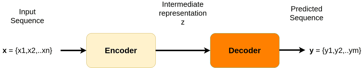
Sequence to sequence learning

Before attention and transformers,Sequence to Sequence (Seq2Seq) worked pretty much like this:

The elements of the sequence $x_1, x_2$, etc. are usually called tokens. They can be literally anything. For instance, text representations, pixels, or even images in the case of videos.

OK. So why do we use such models?

The two sequences can be of the same or arbitrary length.

In case you are wondering, recurrent neural networks (RNNs) dominated this category of tasks. The reason is simple: we liked to treat sequences sequentially. Sounds obvious and optimal? Transformers proved us it’s not!

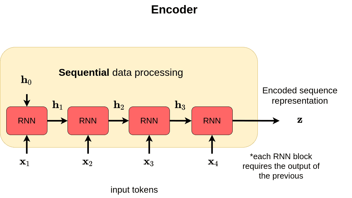
A high-level view of encoder and decoder

The encoder and decoder are nothing more than stacked RNN layers, such as LSTM’s. The encoder processes the input and produces one compact representation, called z, from all the input timesteps. It can be regarded as a compressed format of the input.

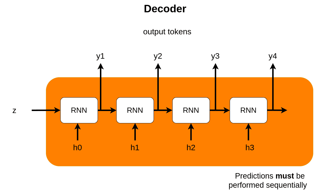
On the other hand, the decoder receives the context vector z and generates the output sequence. The most common application of Seq2seq is language translation. We can think of the input sequence as the representation of a sentence in English and the output as the same sentence in French.

In fact, RNN-based architectures used to work very well especially with LSTM and GRU components.

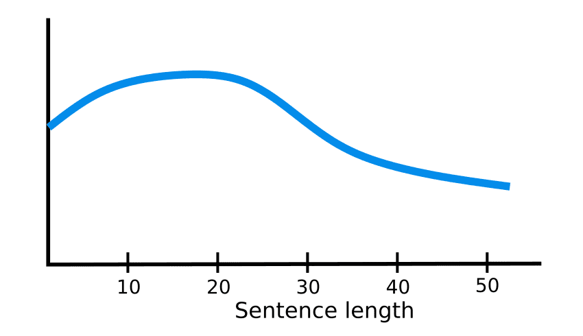
The problem? Only for small sequences (<20 timesteps). Visually:

Let’s inspect some of the reasons why this holds true.

The limitations of RNN’s

The intermediate representation z cannot encode information from all the input timesteps. This is commonly known as the bottleneck problem. The vector z needs to capture all the information about the source sentence.

In theory, mathematics indicate that this is possible. However in practice, how far we can see in the past (the so-called reference window) is finite. RNN’s tend to forget information from timesteps that are far behind.

Let’s see a concrete example. Imagine a sentence of 97 words:

Notice anything wrong? Hmmm… The bold words that facilitate the understanding are quite far!

In most cases, the vector z will be unable to compress the information of the early words as well as the 97th word.

Eventually, the system pays more attention to the last parts of the sequence. However, this is not usually the optimal way to approach a sequence task and it is not compatible with the way humans translate or even understand language.

Furthermore, the stacked RNN layer usually create the well-know vanishing gradient problem, as perfectly visualized in the distill article on RNN’s:

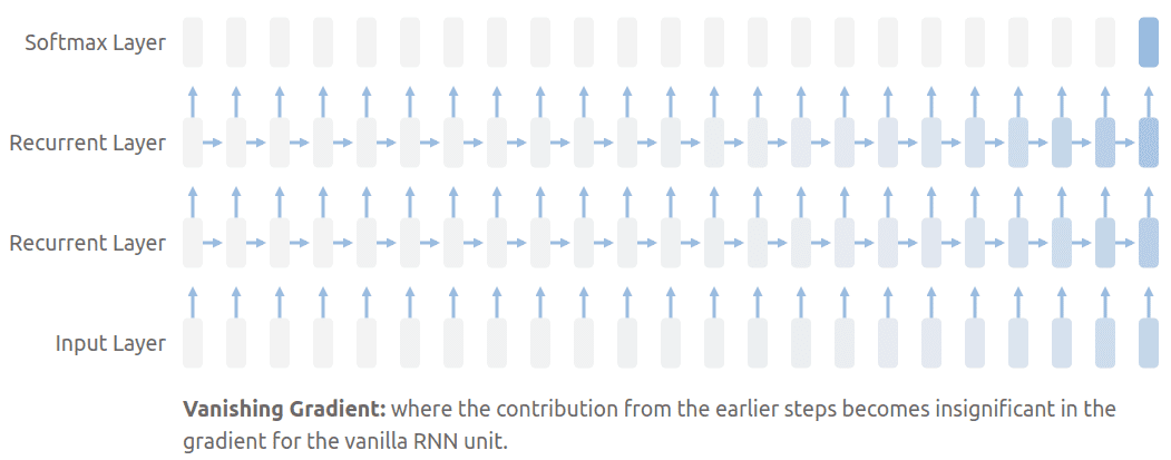The stacked layers in RNN's may result in the vanishing gradient problem. Source

Thus, let us move beyond the standard encoder-decoder RNN.

Attention to the rescue!

Attention was born in order to address these two things on the Seq2seq model. But how?

In other words, we need to form a direct connection with each timestamp.

This idea was originally proposed for computer vision. Larochelle and Hinton [5] proposed that by looking at different parts of the image (glimpses), we can learn to accumulate information about a shape and classify the image accordingly.

The same principle was later extended to sequences. We can look at all the different words at the same time and learn to “pay attention“ to the correct ones depending on the task at hand.

And behold. This is what we now call attention, which is simply a notion of memory, gained from attending at multiple inputs through time.

It is crucial in my humble opinion to understand the generality of this concept. To this end, we will cover all the different types that one can divide attention mechanisms.

Types of attention: implicit VS explicit

Before we continue with a concrete example of how attention is used on machine translation, let’s clarify one thing:

Deep networks are very rich function approximators. So, without any further modification, they tend to ignore parts of the input and focus on others. For instance, when working on human pose estimation, the network will be more sensitive to the pixels of the human body. Here is an example of self-supervised approaches to videos:

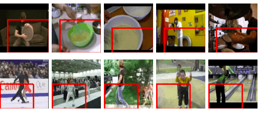Where activations tend to focus when trained in a self-supervised way. Image from Misra et al. ECCV 2016. Source

“Many activation units show a preference for human body parts and pose.” ~ Misra et al. 2016

One way to visualize implicit attention is by looking at the partial derivatives with respect to the input. In math, this is the Jacobian matrix, but it’s out of the scope of this article.

However, we have many reasons to enforce this idea of implicit attention. Attention is quite intuitive and interpretable to the human mind. Thus, by asking the network to ‘weigh’ its sensitivity to the input based on memory from previous inputs, we introduce explicit attention. From now on, we will refer to this as attention.

Types of attention: hard VS soft

Another distinction we tend to make is between hard and soft attention. In all the previous cases, we refer to attention that is parametrized by differentiable functions. For the record, this is termed as soft attention in the literature. Officially:

Historically, we had another concept called hard attention.

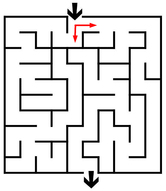
An intuitive example: You can imagine a robot in a labyrinth that has to make a hard decision on which path to take, as indicated by the red dots.

In general, hard means that it can be described by discrete variables while soft attention is described by continuous variables. In other words, hard attention replaces a deterministic method with a stochastic sampling model.

In the next example, starting from a random location in the image tries to find the “important pixels” for classification. Roughly, the algorithm has to choose a direction to go inside the image, during training.

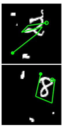An example of hard attention.Source

Since hard attention is non-differentiable, we can’t use the standard gradient descent. That’s why we need to train them using Reinforcement Learning (RL) techniques such as policy gradients and the REINFORCE algorithm [6].

Nevertheless, the major issue with the REINFORCE algorithm and similar RL methods is that they have a high variance. To summarize:

Ultimately, given that we already have all the sequence tokens available, we can relax the definition of hard attention. In this way, we have a smooth differentiable function that we can train end to end with our favorite backpropagation.

Let’s get back to our showcase to see it in action!

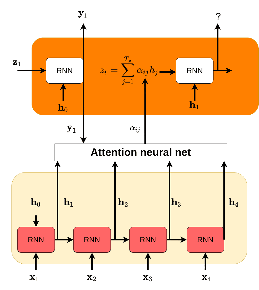
Attention in our encoder-decoder example

In the encoder-decoder RNN case, given previous state in the decoder as $\textbf{y}_{i-1}$ and the the hidden state $\textbf{h} = {h_1,h_2, h_{n} }$, we have something like this:

$$\textbf{e}_{i}=\operatorname{attention_{net}}\left(y_{i-1}, \textbf{h} \right) \in R{^n}$$

The index i indicates the prediction step. Essentially, we define a score between the hidden state of the decoder and all the hidden states of the encoder.

More specifically, for each hidden state (denoted by j) $\textbf{h}_1,\textbf{h}_2,\textbf{h}_n$ we will calculate a scalar:

$$e_{i j}=\operatorname{attention_{net}}\left(\textbf{y}_{i-1}, h_{j}\right)$$

Visually, in our beloved example, we have something like this:

Notice anything strange?

I used the symbol e in the equation and α in the diagram! Why?

Because, we want some extra properties: a) to make it a probability distribution and b) to make the scores to be far from each other. The latter results in having more confident predictions and is nothing more than our well known softmax.

$$\alpha_{i j}=\frac{\exp \left(e_{i j}\right)}{\sum_{k=1}^{T_{x}} \exp \left(e_{i k}\right)}$$

Finally, here is where the new magic will happen:

$$z_{i}=\sum_{j=1}^{T} \alpha_{i j} \textbf{h}_{j}$$

In theory, attention is defined as the weighted average of values. But this time, the weighting is a learned function! Intuitively, we can think of $\alpha_{i j}$ as data-dependent dynamic weights. Therefore, it is obvious that we need a notion of memory, and as we said attention weight store the memory that is gained through time

All the aforementioned are independent of how we choose to model attention! We will get down to that in a bit.

Attention as a trainable weight mean for machine translation

I find that the most intuitive way to understand attention in NLP tasks is to think of it as a (soft) alignment between words. But what does this alignment look like? Excellent question!

In machine translation, we can visualize the attention of a trained network using a heatmap such as below. Note that scores are computed dynamically.

Image by Neural Machine translation paper. Source

Notice what happens in the active non-diagonal elements. In the marked red area, the model learned to swap the order of words in translation. Also note that this is not a 1-1 relationship but a 1 to many, meaning that an output word is affected by more than one input word (each one with different importance).

How do we compute attention?

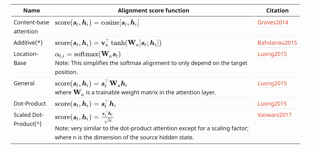
In our previous encoder-decoder example, we denoted attention as $\operatorname{attention_{net}}\left(y_{i-1}, \textbf{h} \right)$ which indicates that it’s the output of a small neural network with inputs the previous state of the decoder as $y_{i-1}$ and the hidden state $h = {h1,h_2, h_{n} }$. In fact all we need is a score that describes the relationship between the two states and captures how “aligned” they are.

While a small neural network is the most prominent approach, over the years there have been many different ideas to compute that score. The simplest one, as shown in Luong [7], computes attention as the dot product between the two states $y_{i-1}\textbf{h}$. Extending this idea we can introduce a trainable weight matrix in between $y_{i-1}W_a\textbf{h}$, where $W_a$ is an intermediate wmatrix with learnable weights. Extending even further, we can also include an activation function in the mix which leads to our familiar neural network approach ${v_a^T}{tanh}(W_a[h; y_{i-1}])$ proposed by Bahdanau [2]

In certain cases, the alignment is only affected by the position of the hidden state, which can be formulated using simply a softmax function $\operatorname{softmax}(y_{i-1},\textbf{h})$

The last one worth mentioning can be found in Graves A. [8] in the context of Neural Turing Machines and calculates attention as a cosine similarity $cosine[y_{i-1},\textbf{h}]$

To summarize the different techniques, I’ll borrow this table from Lillian Weng’s excellent article. The symbol $s_t$ denotes the predictions (I used $y_t$), while different $W$ indicate trainable matrices:

Ways to compute attention. Source

The approach that stood the test of time, however, is the last one proposed by Bahdanau et al. [2]: They parametrize attention as a small fully connected neural network. And obviously, we can extend that to use more layers.

This effectively means that attention is now a set of trainable weights that can be tuned using our standard backpropagation algorithm.

So, what do we lose? Hmm... I am glad you asked!

We sacrificed computational complexity. We have another neural network to train and we need to have $O(T^2)$ weights (where $T$ is the length of both the input and output sentence).

Quadratic complexity can often be a problem! Unless you own Google ;)

And that brings us to local attention.

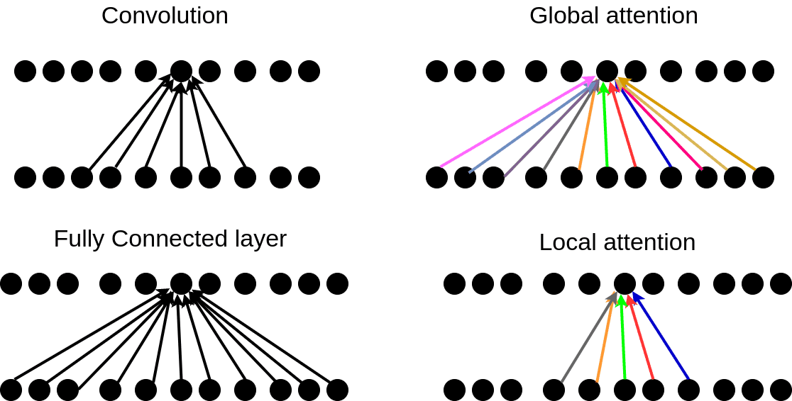
Global vs Local Attention

Until now we assumed that attention is computed over the entire input sequence (global attention). Despite its simplicity, it can be computationally expensive and sometimes unnecessary. As a result, there are papers that suggest local attention as a solution.

"In local attention, we consider only a subset of the input units/tokens."

Evidently, this can sometimes be better for very long sequences. Local attention can also be merely seen as hard attention since we need to take a hard decision first, to exclude some input units.

Let’s wrap up the operations in a simple diagram:

The colors in the attention indicate that these weights are constantly changing while in convolution and fully connected layers they are slowly changing by gradient descent.

The last and undeniably the most famous category is self-attention.

Self-attention: the key component of the Transformer architecture

We can also define the attention of the same sequence, called self-attention. Instead of looking for an input-output sequence association/alignment, we are now looking for scores between the elements of the sequence, as depicted below:

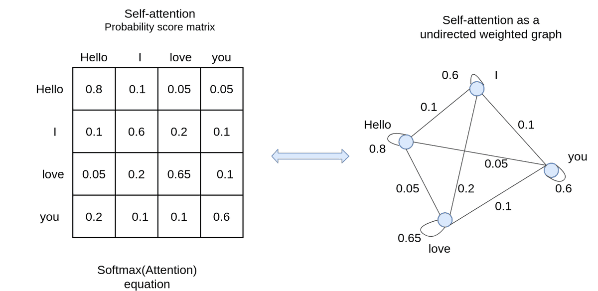
Personally, I like to think of self-attention as a graph. Actually, it can be regarded as a (k-vertex) connected undirected weighted graph. Undirected indicates that the matrix is symmetric.

In maths we have: $\operatorname{self-attention_{net}}\left(x, x \right)$. The self-attention can be computed in any mentioned trainable way. The end goal is to create a meaningful representation of the sequence before transforming to another.

Advantages of Attention

Admittedly, attention has a lot of reasons to be effective apart from tackling the bottleneck problem. First, it usually eliminates the vanishing gradient problem, as they provide direct connections between the encoder states and the decoder. Conceptually, they act similarly as skip connections in convolutional neural networks.

One other aspect that I’m personally very excited about is explainability. By inspecting the distribution of attention weights, we can gain insights into the behavior of the model, as well as to understand its limitations.

Think, for example, the English-to-French heatmap we showed before. I had an aha moment when I saw the swap of words in translation. Don’t tell me that it isn't extremely useful.

Attention beyond language translation

Sequences are everywhere!

While transformers are definitely used for machine translation, they are often considered as general-purpose NLP models that are also effective on tasks like text generation, chatbots, text classification, etc. Just take a look at Google’s BERT or OpenAI’s GPT-3.

But we can also go beyond NLP. We briefly saw attention being used in image classification models, where we look at different parts of an image to solve a specific task. In fact, visual attention models recently outperformed the state of the art Imagenet model [3]. We also have seen examples in healthcare, recommender systems, and even on graph neural networks.

To summarize everything said so far in a nutshell, I would say: Attention is much more than transformers and transformers are more than NLP approaches.

-------------

Source: theaisummer.com

***Thank You***

Share this post