Gradient Boosting

What are Ensemble Techniques ?

Bias and Variance — While building any model, our objective is to optimize both variance and bias but in the real world scenario, one comes at the cost of the other. It is important to understand the trade-off and figure out what suits our use case.

Ensembles are built on the idea that a collection of weak predictors, when combined together, give a final prediction which performs much better than the individual ones. Ensembles can be of two types —

i) Bagging — Bootstrap Aggregation or Bagging is a ML algorithm in which a number of independent predictors are built by taking samples with replacement. The individual outcomes are then combined by average (Regression) or majority voting (Classification) to derive the final prediction. A widely used algorithm in this space is Random Forest.

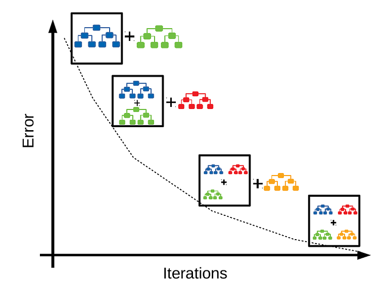
ii) Boosting — Boosting is a ML algorithm in which the weak learners are converted into strong learners. Weak learners are classifiers which always perform slightly better than chance irrespective of the distribution over the training data. In Boosting, the predictions are sequential wherein each subsequent predictor learns from the errors of the previous predictors. Gradient Boosting Trees (GBT) is a commonly used method in this category.

Performance comparison of these two methods in reducing Bias and Variance — Bagging has many uncorrelated trees in the final model which helps in reducing variance. Boosting will reduce variance in the process of building sequential trees. At the same time, its focus remains on bridging the gap between the actual and predicted values by reducing residuals, hence it also reduces bias.

Gradient Boosting

Gradient Boosting relies on the intuition that the best possible next model , when combined with the previous models, minimizes the overall prediction errors. The key idea is to set the target outcomes from the previous models to the next model in order to minimize the errors. This is another boosting algorithm(few others are Adaboost, XGBoost etc.).

Input requirement for Gradient Boosting:

1. A Loss Function to optimize.
2. A weak learner to make prediction(Generally Decision tree).
3. An additive model to add weak learners to minimize the loss function.

1. Loss Function

The loss function basically tells how my algorithm, models the data set.In simple terms it is difference between actual values and predicted values.

Regression Loss functions:

1. L1 loss or Mean Absolute Errors (MAE)
2. L2 Loss or Mean Square Error(MSE)
3. Quadratic Loss

Binary Classification Loss Functions:

1. Binary Cross Entropy Loss
2. Hinge Loss

A gradient descent procedure is used to minimize the loss when adding trees.

2. Weak Learner

Weak learners are the models which is used sequentially to reduce the error generated from the previous models and to return a strong model on the end.

Decision trees are used as weak learner in gradient boosting algorithm.

3. Additive Model

In gradient boosting, decision trees are added one at a time (in sequence), and existing trees in the model are not changed.

Understanding Gradient Boosting Step by Step :

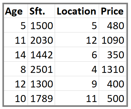
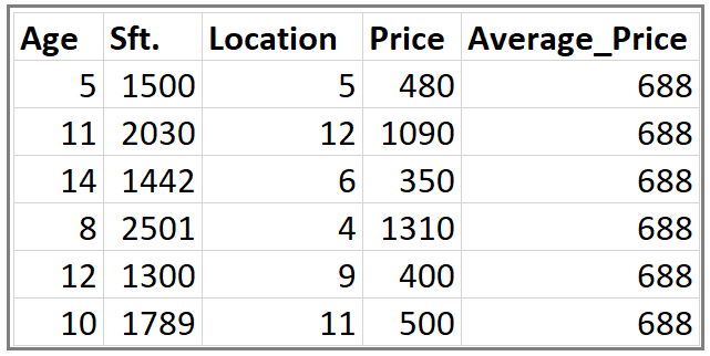
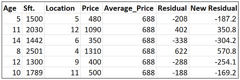
This is our data set. Here Age, Sft., Location is independent variables and Price is dependent variable or Target variable.

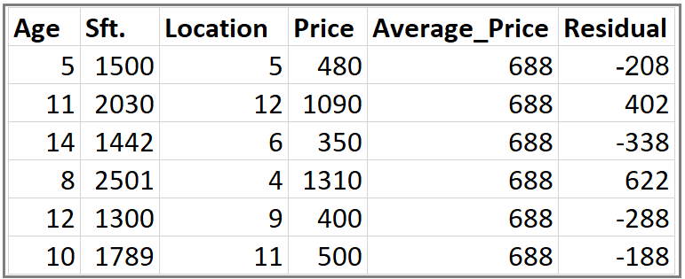
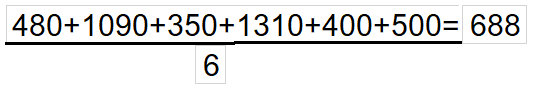
Step 1: Calculate the average/mean of the target variable.

Step 2: Calculate the residuals for each sample.

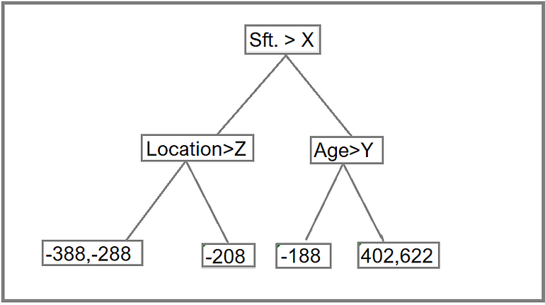
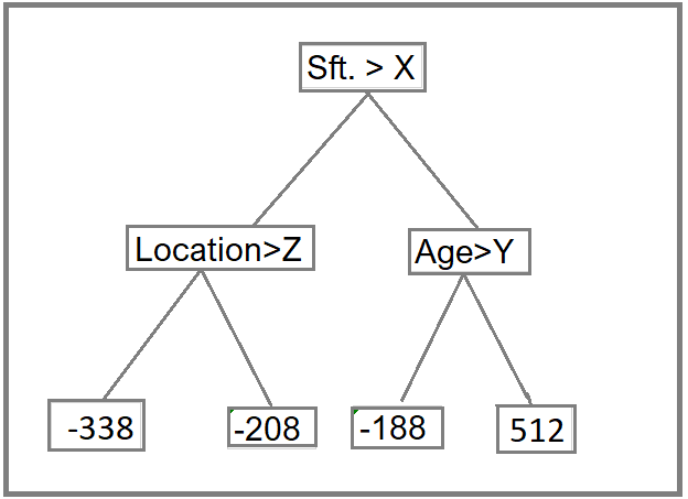
Step 3: Construct a decision tree. We build a tree with the goal of predicting the Residuals.

In the event if there are more residuals then leaf nodes(here its 6 residuals),some residuals will end up inside the same leaf. When this happens, we compute their average and place that inside the leaf.

      

 

After this tree become like this.

Step 4: Predict the target label using all the trees within the ensemble.

Each sample passes through the decision nodes of the newly formed tree until it reaches a given lead. The residual in the said leaf is used to predict the house price.

         

         

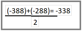
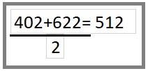
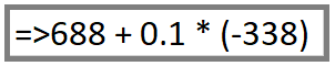
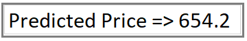
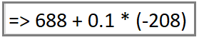
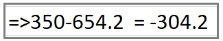
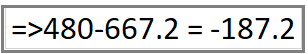
Calculation above for Residual value (-338) and (-208) in Step 2

Same way we will calculate the Predicted Price for other values

Note: We have initially taken 0.1 as learning rate.

Step 5 : Compute the new residuals

When Price is 350 and 480 Respectively.

With our Single leaf with average value(688) we have the below column of Residual

With our decision tree ,we ended up the below new residuals

Step 6: Repeat steps 3 to 5 until the number of iterations matches the number specified by the hyper parameter(numbers of estimators)

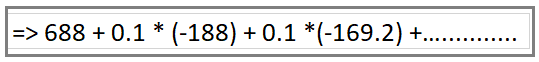
Step 7: Once trained, use all of the trees in the ensemble to make a final prediction as to value of the target variable. The final prediction will be equal to the mean we computed in Step 1 plus all the residuals predicted by the trees that make up the forest multiplied by the learning rate.

Here,

LR : Learning Rate

DT: Decision Tree

Important Parameters

While constructing any model using GBTree, the values of the following can be tweaked for improvement in model performance -

• number of trees (n_estimators; def: 100)
• learning rate (learning_rate; def: 0.1) — Scales the contribution of each tree as discussed before. There is a trade-off between learning rate and number of trees. Commonly used values of learning rate lie between 0.1 to 0.3
• maximum depth (max_depth; def: 3) — Maximum depth of each estimator. It limits the number of nodes of the decision trees

Note — The names of these parameters in Python environment along with their default values are mentioned within brackets

Advantages of Gradient Boosting

1. Most of the time predictive accuracy of gradient boosting algorithm on higher side.
2. It provides lots of flexibility and can optimize on different loss functions and provides several hyper parameter tuning options that make the function fit very flexible.
3. Most of the time no data pre-processing required.
4. Gradient Boosting algorithm works great with categorical and numerical data.
5. Handles missing data — missing value imputation not required.

Disadvantages of Gradient Boosting

1. Gradient Boosting Models will continue improving to minimize all errors. This can overemphasize outliers and cause over fitting. Must use cross-validation to neutralize.
2. It is computationally very expensive — GBMs often require many trees (>1000) which can be time and memory exhaustive.
3. The high flexibility results in many parameters that interact and influence heavily the behavior of the approach (number of iterations, tree depth, regularization parameters, etc.). This requires a large grid search during tuning.

Conclusion

Gradient Boosting algorithm is very widely used machine learning and predictive modeling technique (Preferred in Kaggle and other code competitions).

***Thank You***

Share this post