Dimensionality Reduction

In both Statistics and Machine Learning, the number of attributes, features or input variables of a dataset is referred to as its dimensionality. For example, let’s take a very simple dataset containing 2 attributes called Height and Weight. This is a 2-dimensional dataset and any observation of this dataset can be plotted in a 2D plot.

If we add another dimension called Age to the same dataset, it becomes a 3-dimensional dataset and any observation lies in the 3-dimensional space.

Likewise, real-world datasets have many attributes. The observations of those datasets lie in high-dimensional space which is hard to imagine. The following is a general geometric interpretation of a dataset related to dimensionality considered by data scientists, statisticians and machine learning engineers.

"In a tabular dataset containing rows and columns, the columns represent the dimensions of the n-dimensional feature space and the rows are the data points lying in that space".

Dimensionality reduction simply refers to the process of reducing the number of attributes in a dataset while keeping as much of the variation in the original dataset as possible. It is a data preprocessing step meaning that we perform dimensionality reduction before training the model. In this article, we will discuss 11 such dimensionality reduction techniques and implement them with real-world datasets using Python and Scikit-learn libraries.

The importance of dimensionality reduction

When we reduce the dimensionality of a dataset, we lose some percentage (usually 1%-15% depending on the number of components or features that we keep) of the variability in the original data. But, don’t worry about losing that much percentage of the variability in the original data because dimensionality reduction will lead to the following advantages.

• A lower number of dimensions in data means less training time and less computational resources and increases the overall performance of machine learning algorithms — Machine learning problems that involve many features make training extremely slow. Most data points in high-dimensional space are very close to the border of that space. This is because there’s plenty of space in high dimensions. In a high-dimensional dataset, most data points are likely to be far away from each other. Therefore, the algorithms cannot effectively and efficiently train on the high-dimensional data. In machine learning, that kind of problem is referred to as the curse of dimensionality — this is just a technical term that you do not need to worry about!
• Dimensionality reduction avoids the problem of overfitting — When there are many features in the data, the models become more complex and tend to overfit on the training data.
• Dimensionality reduction is extremely useful for data visualization — When we reduce the dimensionality of higher dimensional data into two or three components, then the data can easily be plotted on a 2D or 3D plot.
• Dimensionality reduction takes care of multicollinearity — In regression, multicollinearity occurs when an independent variable is highly correlated with one or more of the other independent variables. Dimensionality reduction takes advantage of this and combines those highly correlated variables into a set of uncorrelated variables. This will address the problem of multicollinearity.
• Dimensionality reduction is very useful for factor analysis — This is a useful approach to find latent variables which are not directly measured in a single variable but rather inferred from other variables in the dataset. These latent variables are called factors.
• Dimensionality reduction removes noise in the data — By keeping only the most important features and removing the redundant features, dimensionality reduction removes noise in the data. This will improve the model accuracy.
• Dimensionality reduction can be used for image compression — image compression is a technique that minimizes the size in bytes of an image while keeping as much of the quality of the image as possible. The pixels which make the image can be considered as dimensions (columns/variables) of the image data. We perform PCA to keep an optimum number of components that balance the explained variability in the image data and the image quality.
• Dimensionality reduction can be used to transform non-linear data into a linearly-separable form.

Dimensionality reduction methods :

There are several dimensionality reduction methods that can be used with different types of data for different requirements. The following chart summarizes those dimensionality reduction methods.

There are mainly two types of dimensionality reduction methods. Both methods reduce the number of dimensions but in different ways. It is very important to distinguish between those two types of methods. One type of method only keeps the most important features in the dataset and removes the redundant features. There is no transformation applied to the set of features. Backward elimination, Forward selection and Random forests are examples of this method. The other method finds a combination of new features. An appropriate transformation is applied to the set of features. The new set of features contains different values instead of the original values. This method can be further divided into Linear methods and Non-linear methods. Non-linear methods are well known as Manifold learning. Principal Component Analysis (PCA), Factor Analysis (FA), Linear Discriminant Analysis (LDA) and Truncated Singular Value Decomposition (SVD) are examples of linear dimensionality reduction methods. Kernel PCA, t-distributed Stochastic Neighbor Embedding (t-SNE), Multidimensional Scaling (MDS) and Isometric mapping (Isomap) are examples of non-linear dimensionality reduction methods.Let’s discuss each method in detail.

Linear methods

Linear methods involve linearly projecting the original data onto a low-dimensional space. We’ll discuss PCA, FA, LDA and Truncated SVD under linear methods. These methods can be applied to linear data and do not perform well on non-linear data.

Principal Component Analysis (PCA)

PCA is a linear dimensionality reduction technique (algorithm) that transforms a set of correlated variables (p) into a smaller k (k<p) number of uncorrelated variables called principal components while retaining as much of the variation in the original dataset as possible. In the context of Machine Learning (ML), PCA is an unsupervised machine learning algorithm that is used for dimensionality reduction.

Factor Analysis (FA)

Factor Analysis (FA) and Principal Component Analysis (PCA) are both dimensionality reduction techniques. The main objective of Factor Analysis is not to just reduce the dimensionality of the data. Factor Analysis is a useful approach to find latent variables which are not directly measured in a single variable but rather inferred from other variables in the dataset. These latent variables are called factors.

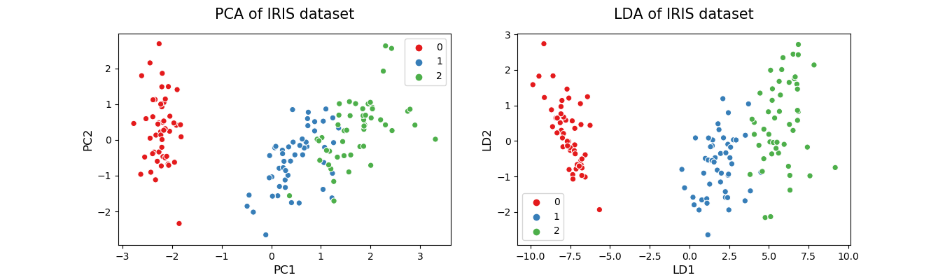
Linear Discriminant Analysis (LDA)

LDA is typically used for multi-class classification. It can also be used as a dimensionality reduction technique. LDA best separates or discriminates (hence the name LDA) training instances by their classes. The major difference between LDA and PCA is that LDA finds a linear combination of input features that optimizes class separability while PCA attempts to find a set of uncorrelated components of maximum variance in a dataset. Another key difference between the two is that PCA is an unsupervised algorithm whereas LDA is a supervised algorithm where it takes class labels into account.

There are some limitations of LDA. To apply LDA, the data should be normally distributed. The dataset should also contain known class labels. The maximum number of components that LDA can find is the number of classes minus 1. If there are only 3 class labels in your dataset, LDA can find only 2 (3–1) components in dimensionality reduction. It is not needed to perform feature scaling to apply LDA. On the other hand, PCA needs scaled data. However, class labels are not needed for PCA. The maximum number of components that PCA can find is the number of input features in the original dataset.

LDA for dimensionality reduction should not be confused with LDA for multi-class classification. Both cases can be implemented using the Scikit-learn LinearDiscriminantAnalysis() function. After fitting the model using fit(X, y), we use the predict(X) method of the LDA object for multi-class classification. This will assign new instances to the classes in the original dataset. We can use the transform(X) method of the LDA object for dimensionality reduction. This will find a linear combination of new features that optimizes class separability.

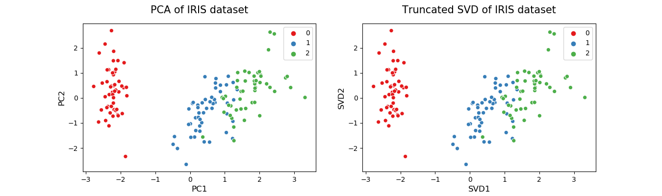
Truncated Singular Value Decomposition (SVD)

This method performs linear dimensionality reduction by means of truncated singular value decomposition (SVD). It works well with sparse data in which many of the row values are zero. In contrast, PCA works well with dense data. Truncated SVD can also be used with dense data. Another key difference between truncated SVD and PCA is that factorization for SVD is done on the data matrix while factorization for PCA is done on the covariance matrix.

Non-linear methods (Manifold learning)

If we’re dealing with non-linear data which are frequently used in real-world applications, linear methods discussed so far do not perform well for dimensionality reduction. In this section, we’ll discuss four non-linear dimensionality reduction methods that can be used with non-linear data.

Kernel PCA

Kernel PCA is a non-linear dimensionality reduction technique that uses kernels. It can also be considered as the non-linear form of normal PCA. Kernel PCA works well with non-linear datasets where normal PCA cannot be used efficiently.

The intuition behind Kernel PCA is something interesting. The data is first run through a kernel function and temporarily projects them into a new higher-dimensional feature space where the classes become linearly separable (classes can be divided by drawing a straight line). Then the algorithm uses the normal PCA to project the data back onto a lower-dimensional space. In this way, Kernel PCA transforms non-linear data into a lower-dimensional space of data which can be used with linear classifiers.

In the Kernel PCA, we need to specify 3 important hyperparameters — the number of components we want to keep, the type of kernel and the kernel coefficient (also known as the gamma). For the type of kernel, we can use ‘linear’, ‘poly’, ‘rbf’, ‘sigmoid’, ‘cosine’. The rbf kernel which is known as the radial basis function kernel is the most popular one.

One limitation of using the Kernel PCA for dimensionality reduction is that we have to specify a value for the gamma hyperparameter before running the algorithm. It requires implementing a hyperparameter tuning technique such as Grid Search to find an optimal value for the gamma. It is beyond the scope of this article.

t-distributed Stochastic Neighbor Embedding (t-SNE)

This is also a non-linear dimensionality reduction method mostly used for data visualization. In addition to that, it is widely used in image processing and NLP. The Scikit-learn documentation recommends you to use PCA or Truncated SVD before t-SNE if the number of features in the dataset is more than 50. 

Multidimensional Scaling (MDS)

MDA is another non-linear dimensionality reduction technique that tries to preserve the distances between instances while reducing the dimensionality of non-linear data. There are two types of MDS algorithms: Metric and Non-metric. The MDS() class in the Scikit-learn implements both by setting the metric hyperparameter to True (for Metric type) or False (for Non-metric type).

Isometric mapping (Isomap)

This method performs non-linear dimensionality reduction through Isometric mapping. It is an extension of MDS or Kernel PCA. It connects each instance by calculating the curved or geodesic distance to its nearest neighbors and reduces dimensionality. The number of neighbors to consider for each point can be specified through the n_neighbors hyperparameter of the Isomap() class which implements the Isomap algorithm in the Scikit-learn.

Other methods

Under this category, we’ll discuss 3 methods. Those methods only keep the most important features in the dataset and remove the redundant features. So, they are mainly used for feature selection. But, dimensionality reduction happens automatically while selecting the best features! Therefore, they can also be considered dimensionality reduction methods. These methods will improve models’ accuracy scores or boost performance on very high-dimensional datasets.

Backward Elimination

This method eliminates (removes) features from a dataset through a recursive feature elimination (RFE) process. The algorithm first attempts to train the model on the initial set of features in the dataset and calculates the performance of the model (usually, accuracy score for a classification model and RMSE for a regression model). Then, the algorithm drops one feature (variable) at a time, trains the model on the remaining features and calculates the performance scores. The algorithm repeats eliminating features until it detects a small (or no) change in the performance score of the model and stops there!

In the Scikit-learn, backward elimination can be implemented by using the RFE() class which is in the sklearn.feature_selection module. The first parameter of that class should be a supervised learning estimator with a fit() method and a coef_ or feature_importances_ attribute. The second one should be the number of features to select. According to the Scikit-learn documentation, half of the features are selected if we do not specify the number of features to select (n_features_to_select parameter). A major limitation of this method is that we do not know the number of features to select. In those situations, it is better to run this algorithm multiple times by specifying different values for n_features_to_select.

Forward Selection

This method can be considered as the opposite process of backward elimination. Instead of eliminating features recursively, the algorithm attempts to train the model on a single feature in the dataset and calculates the performance of the model (usually, accuracy score for a classification model and RMSE for a regression model). Then, the algorithm adds (selects) one feature (variable) at a time, trains the model on those features and calculates the performance scores. The algorithm repeats adding features until it detects a small (or no) change in the performance score of the model and stops there!

In Scikit-learn, there is no direct function for forward feature selection. Instead, we can use f_regression (for regression tasks) and f_classif (for classification tasks) classes together with the SelectKBest class. f_regression returns F-value between label/feature for regression tasks. f_classif returns ANOVA F-value between label/feature for classification tasks. Those F-values can be used in the feature selection process. The SelectKBest automatically selects features according to the highest scores based on the F-values of features. The score_func parameter of SelectKBest should be specified to f_classif or f_regression. The k parameter defines the number of top features to select.

Random forests

Random forests is a tree-based model which is widely used for regression and classification tasks on non-linear data. It can also be used for feature selection with its built-in feature_importances_ attribute which calculates feature importance scores for each feature based on the ‘gini’ criterion (a measure of the quality of a split of internal nodes) while training the model.

***Thank You***

Share this post