Logistic Regression

Logistic Regression

While Linear Regression is used to predict the continuous value of a dependent variable, Logistic Regression is a classification algorithm.It is used to predict something which is true or false(binary classification).

Types of Logistic Regression:

Binomial Logistic Regression

Used for Binary Classification: The target variable can have only 2 possible outcomes like 0 or 1 which represent Obese/Not Obese, Dead/Alive, Spam/Not Spam, etc…

Multinomial Logistic Regression

Used for Multi-class Classification: The target variable can have 3 or more possible outcomes e.g. Disease A/Disease B/Disease C or Digit Classification, etc...

Logistic is abbreviated from the Logit function and its working is quite similar to that of a Linear Regression algorithm hence the name Logistic Regression.

Note: Logistic Regression becomes a classification technique only when a decision threshold is brought into the picture i.e. If the decision threshold is not taken into consideration then Logistic Regression would become a regression model that regresses/predicts the probability of a given input data.

The setting of the threshold value (default = 0.5) is a very important aspect of Logistic Regression and is dependent on the classification problem itself.

Working of Logistic Regression:

Consider an example of classifying a patient is obese or not obese where if the output is 1 means the patient is obese and 0 means not obese.

Note: As Linear Regression uses the Ordinary Least Squares (OLE) method to select its best fit line, this can’t be done in the case of Logistic Regression and to know why; watch this video. Instead, Logistic Regression uses Maximum Likelihood to select the best fit line.

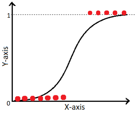
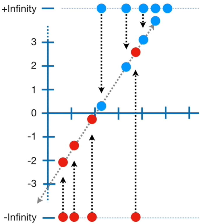
The Logistic Regression model firstly converts the probability into a log(odds) or log of odds as we call it, as shown in the figure below.

        

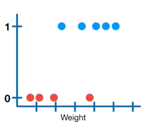
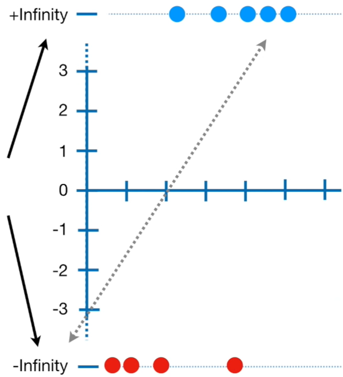
Note: The y-axis of the left image consists of probability ranging from 0 to 1 with a default threshold value of 0.5 and the y-axis of the right image consists of the log(odds) values ranging from +infinity to -infinity. The conversion from probability to log(odds) is done using the logit function.

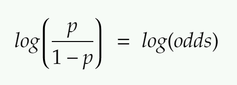
Note: If we use the default threshold value = 0.5 and substitute in the above equation, we will end up with log(odds) = 0 which is the center of the log(odds) graph. Similarly, substituting 1 would give us the answer as +infinity whereas substituting 0 would give us the answer as -infinity.

Explanation of log(odds)

To find the log(odds) value for each candidate, we project them onto the line as shown below.

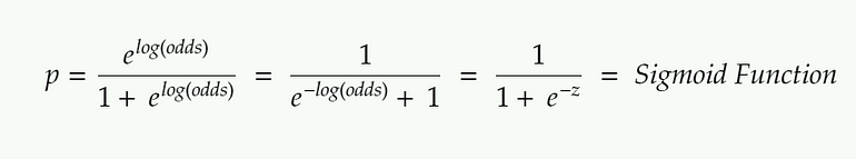
Once we find the log(odds) value for each candidate, we’ll convert back the log(odds) of each candidate to probability using the formula given below. (Sigmoid Function).

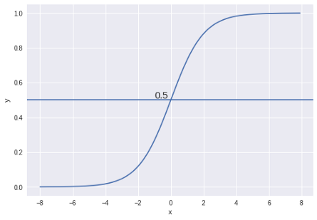
Sigmoid Function with decision threshold = 0.5

What is the Maximum Likelihood Estimation?

The Maximum Likelihood Estimation (MLE) is a likelihood maximization method, while the Ordinary Least Squares (OLS) is a residual minimizing method.

Maximizing the likelihood function determines the parameters that are most likely to produce the observed data. Hence maximum likelihood is used to select the best fit line.

The likelihood, in this case, is the product of probabilities of all the data points being obese and not obese.

On finding the likelihood for the first line, we then rotate the log(odds) line by a bit and again calculate the likelihood. This is done using the Gradient Descent algorithm.

Gradient Descent and Cost Function in Logistic Regression

If you remember, the cost function in Linear Regression looks like.

If you try to use the linear regression’s cost function to generate J(θ) in a logistic regression problem, you would end up with a non-convex function which has many local minimums: a weirdly-shaped graph with no easy to find the minimum global point, as seen in the picture below.

Non-convex function

For logistic regression, the Cost function is defined as follows.

Logistic Regression: Cost Function 

We use this cost function to generate J(θ), which will give us the following graphs.

Convex functions

Repeat the process until the best-fit log(odds) line is found.

Sigmoid Curve (Probability) and Log(odds) line

Note: The coefficients that the logistic regression model shows using classifier.coeff_ the method is for the log(odds) line and not of the sigmoid curve.

This is how Logistic Regression works! 

***Thank You***

Share this post