Linear Regression

Linear Regression

Everyone who are on the track of machine learning or data science might have encounter that the first algorithm they learn is Linear Regression.

Linear Regression is one of the most fundamental algorithms used to model relationships between a dependent variable and one or more independent variables. In simpler terms, it involves finding the ‘line of best fit’ that represents two or more variables.It is used to estimate real values (cost of houses, number of calls, total sales etc.) based on continuous variable(s). Here, we establish relationship between independent and dependent variables by fitting a best line.

This best fit line is known as regression line and represented by a linear equation

Y= m *X + c

In this equation:

Y – Dependent Variable

m – Slope

X – Independent variable

c– Intercept

These coefficients m and c are derived based on minimizing the sum of squared difference of distance between data points and regression line.

The line of best fit is found by minimizing the squared distances between the points and the line of best fit — this is known as minimizing the sum of squared residuals. A residual is simply equal to the predicted value minus the actual value.

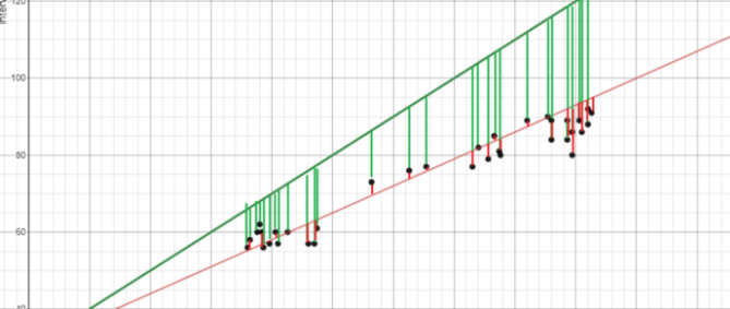
In the above image we can see that the points are closer to the red line than the green line. So the best fit line is the red line.We call that line as Best Fit Line or Regression Line.

What does ‘m’ denote?

If m > 0, then X (predictor) and Y (target) have a positive relationship. This means the value of Y will increase with an increase in the value of X.
If m < 0, then X (predictor) and Y (target) have a negative relationship. This means the value of Y will decrease with an increase in the value of X.

What does ‘c’ denote?

It is the value of Y when X=0. Suppose, if we plot a graph in which the X-axis consists of Years of Experience (independent feature) and Y-axis consists of Salary (dependent feature). For Years of Experience = 0 what will be the Salary, this is what is denoted by ‘c’.

Now that you have understood the theory about the regression line, let’s discuss how can we select the best-fit regression line for a particular model using loss functions.

What is a Loss function?

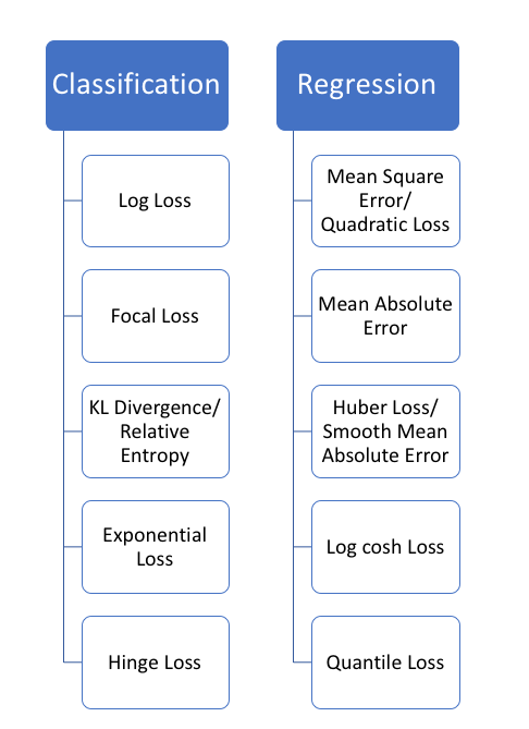
The loss function is the function that computes the distance between the current output of the algorithm and the expected output. It’s a method to evaluate how your algorithm models the data. It can be categorized into two groups. One for classification (discrete values, 0,1,2…) and the other for regression (continuous values).

The terms cost and loss functions almost refer to the same thing. The cost function is calculated as an average of the loss function. The loss function is a value which is calculated at every instance. So, for a single training cycle loss is calculated numerous times, but the cost function is only calculated once.

Note: For algorithms relying on Gradient descent to optimize model parameters, every loss function selected has to be differentiable.

Consider the loss function to be Mean Squared Error (MSE) in our case. Figure 4 shows the formula of this loss function where n is the number of samples in the dataset, Y is the actual value and Ŷ is the corresponding predicted value for iᵗʰ data point.

What is Gradient Descent?

Gradient descent is an iterative optimization algorithm to find the minimum of a function. Here, that function refers to the Loss function.

Also on using Gradient descent, the term learning rate comes into the picture. The learning rate is denoted by α and this parameter controls how much the value of m and c should change after each iteration/step. Selecting the proper value of α is also important as shown in figure.

Starting with an initial value of m and c as 0.0 and setting a small value for the learning rate e.g. α=0.001, for this value we calculate the error value using our loss function. For different values of m and c, we will get different error values as shown in figure.

Once the initial values are selected, we then find the partial derivative of the loss function by applying the chain rule.

Once the slope is calculated, we now update the value of m and c using the formula shown in figure.

If the slope at the particular point is negative then the value of m and c increases and the point shifts towards the right side by a small distance as seen in below figure.
If the slope at the particular point is positive then the value of m and c decreases and the point shifts towards the left side by a small distance.

*****

Multiple Linear Regression:

In real-life scenarios, there will never be a single feature that predicts a target. Hence, we simply perform multiple linear regression.

The equation in below figure shows very similar to the equation for simple linear regression; simply add the number of independent features/predictors and their corresponding coefficients.

Note: The working of the algorithm remains the same, the only thing that changes is the Gradient Descent graph. In Simple Linear Regression, the gradient descent graph was in 2D form, but as the number of independent features/predictors increases, the gradient descent graph’s dimensions also keep on increasing.

Below figure shows a Gradient Descent graph in a 3D format where A is the initial weight/starting point and B is the global minima.

Below figure shows the complete working of the Gradient Descent in 3D format from A to B.

Assumptions of Linear Regression:

The following are the fundamental assumptions of Linear Regression, which can be used to answer the question of whether we can use a linear regression algorithm on a particular dataset?

A linear relationship between features and the target variable:

Linear Regression assumes that the relationship between independent features and the target is linear. It does not support anything else. You may need to transform data to make the relationship linear (e.g. log transform for an exponential relationship).

Little or No Multicollinearity between features:

Multicollinearity exists when the independent variables are found to be moderately or highly correlated. In a model with correlated variables, it becomes a tough task to figure out the true relationship of predictors with the target variable. In other words, it becomes difficult to find out which variable is actually contributing to predict the response variable.

Little or No Autocorrelation in residuals:

The presence of correlation in error terms drastically reduces the model’s accuracy. This usually occurs in time series models where the next instant is dependent on the previous instant. If the error terms are correlated, the estimated standard errors tend to underestimate the true standard error.

No Heteroscedasticity:

The presence of non-constant variance in the error terms results in heteroscedasticity. Generally, non-constant variance arises in the presence of outliers. Looks like, these values get too much weight, thereby disproportionately influences the model’s performance.

Normal distribution of error terms:

If the error terms are not normally distributed, confidence intervals may become too wide or narrow. Once the confidence interval becomes unstable, it leads to difficulty in estimating coefficients based on the least-squares. The presence of non-normal distribution suggests that there are a few unusual data points that must be studied closely to make a better model.