Naive Bayes

 Naive Bayes

Naive Bayes is Supervised Classification algorithm 

This algorithm is called “Naive” because it makes a naive assumption that each feature is independent of other features which is not true in real life.

As for the “Bayes” part, it refers to the statistician and philosopher, Thomas Bayes and the theorem named after him, Bayes’ theorem, which is the base for Naive Bayes Algorithm.

What is Naive Bayes Algorithm?

On Summarizing the above mentioned points Naive Bayes algorithm can be defined as a supervised classification algorithm which is based on Bayes theorem with an assumption of independence among features.

A Brief look on Bayes Theorem :

Bayes Theorem helps us to find the probability of a hypothesis given our prior knowledge.

As per wikipedia,In probability theory and statistics, Bayes’ theorem (alternatively Bayes’ law or Bayes’ rule, also written as Bayes’s theorem) describes the probability of an event, based on prior knowledge of conditions that might be related to the event.

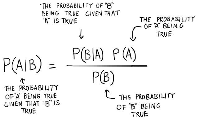
Lets look at the equation for Bayes Theorem,

Where,

P(A|B) is the probability of hypothesis A given the data B. This is called the posterior probability.

P(B|A) is the probability of data B given that the hypothesis A was true.

P(A) is the probability of hypothesis A being true (regardless of the data). This is called the prior probability of A.

P(B) is the probability of the data (regardless of the hypothesis).

If you are thinking what is P(A|B) or P(B|A)?These are conditional probabilities having formula :

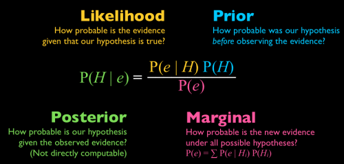
If you still have confusion,this image summarizes Bayes Theorem-

How does Naive Bayes Algorithm work?

Example 1: 

Let us take an example to understand how does Naive Bayes Algorithm work.

Suppose we have a training dataset of 1025 fruits.The feature in the dataset are these : Yellow_color,Big_Size,Sweet_Taste.There are three different classes apple,banana & others.

Step 1: Create a frequency table for all features against all classes

What can we conclude from the above table?

Out of 1025 fruits, 400 are apples, 525 are bananas, and 100 are others.

175 of the total 400 apples are Yellow and the rest are not and so on.

400 fruits are Yellow, 425 are big in size and 200 are sweet from a total of 600 fruits.

Step 2: Draw the likelihood table for the features against the classes.

In our likelihood table Total_Probability of banana is maximum(0.1544) when the fruit is of Yellow_Color,Big in size and Sweet in taste.Therefore as per Naive Bayes algorithm a fruit which is Yellow in color,big in size and sweet in taste is Banana.

In a nutshell, we say that a new element will belong to the class which will have the maximum conditional probability described above.

Example 2 :

Assume we have a bunch of emails that we want to classify as spam or not spam.

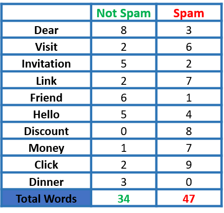
Our dataset has 15 Not Spam emails and 10 Spam emails. Some analysis had been done, and the frequency of each word had been recorded as shown below:

Note: Stop Words like “the”, “a”, “on”, “is”, “all” had been removed as they do not carry important meaning and are usually removed from texts. The same thing applies to numbers and punctuations.

Exploring some probabilities:

P(Dear|Not Spam) = 8/34

P(Visit|Not Spam) = 2/34

P(Dear|Spam) = 3/47

P(Visit|Spam) = 6/47

and so on.

now assume we have the message “Hello friend” and we want to know whether it is a spam or not.

so, using Bayes’ Theorem

ignoring the denominator

But, P(Hello friend | Not Spam) = 0, as this case (Hello friend) doesn’t exist in our dataset, i.e. we deal with single words, not the whole sentence, and the same for P(Hello friend | Spam) will be zero as well, which in turn will make both probabilities of being a spam and not spam both are zero, which has no meaning!!

But wait!! we said that the Naive Bayes assumes that `the features we use to predict the target are independent`.

so,

now let’s calculate the probability of being spam using the same procedure:

so, the message “Hello friend” is not a spam.

now, let’s try another example:

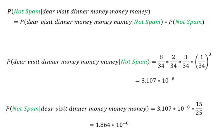
assume the message “dear visit dinner money money money”. It’s obvious that it’s a spam, but let’s see what Naive Bayes will say.

oops!! Naive Bays says that this message is not a spam?!!!

This happened because the word “dinner” does not appear in the spam dataset, so that P(dinner | spam) = 0, hence all other probabilities will have no effect.

This is called the Zero-Frequency Problem.

and to solve that we can use Laplace smoothing.

Laplace Smoothing is a technique for smoothing categorical data. A small-sample correction, or pseudo-count, will be incorporated in every probability estimate. Hence, no probability will be zero. this is a way of regularizing Naive Bayes.

Given an observation x = (x1, …, xd) from a multinomial distribution with N trials and parameter vector θ = (θ1, …, θd), a “smoothed” version of the data gives the estimator:

where the pseudo-count α > 0 is the smoothing parameter (α = 0 corresponds to no smoothing).

Read more about Additive Smoothing here.

Back to our problem, we are going to pick α = 1, and ‘d’ is the number of the unique words in the dataset which is 10 in our case

Now it’s correctly classified the message as spam.

Types of Naive Bayes Classifiers

Multinomial: Feature vectors represent the frequencies with which certain events have been generated by a multinomial distribution. For example, the count how often each word occurs in the document. This is the event model typically used for document classification.

Bernoulli: Like the multinomial model, this model is popular for document classification tasks, where binary term occurrence(i.e. a word occurs in a document or not) features are used rather than term frequencies(i.e. frequency of a word in the document).

Gaussian: It is used in classification and it assumes that features follow a normal distribution.

Pros and Cons for Naive Bayes

Pros:

• Requires a small amount of training data. So the training takes less time.
• Handles continuous and discrete data, and it is not sensitive to irrelevant features.
• Very simple, fast, and easy to implement.
• Can be used for both binary and multi-class classification problems.
• Highly scalable as it scales linearly with the number of predictor features and data points.
• When the Naive Bayes conditional independence assumption holds true, it will converge quicker than discriminative models like logistic regression.

Cons:

• The assumption of independent predictors/features. Naive Bayes implicitly assumes that all the attributes are mutually independent which is almost impossible to find in real-world data.
• If a categorical variable has a value that appears in the test dataset, and not observed in the training dataset, then the model will assign it a zero probability and will not be able to make a prediction. This is what we called the “Zero Frequency problem“, and can be solved using smoothing techniques.

Applications of Naive Bayes Algorithm

• Real-time Prediction.
• Multi-class Prediction.
• Text classification/ Spam Filtering/ Sentiment Analysis.
• Recommendation Systems.

***Thank You***

Share this post