
SUPPORT VECTOR MACHINE BASIC TERMINOLOGY
Vector: This is simply the training examples/data points. It is also known as ‘Feature vectors’ in machine learning.
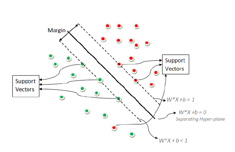
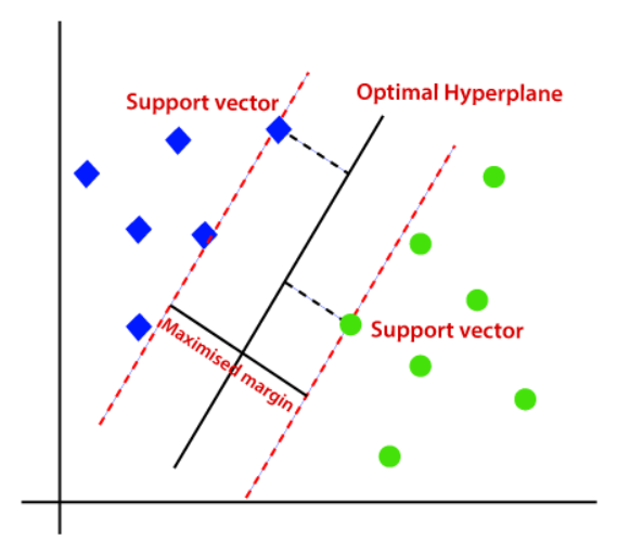
Support + Vector: This is simply a subset of the data closest to the hyperplane/decision boundary.
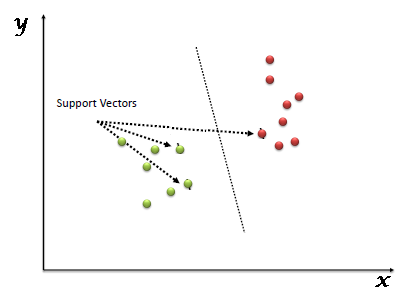
These vectors are intuitively called ‘Support vectors’ because they support the hyperplane/decision boundary and act as a pillar.
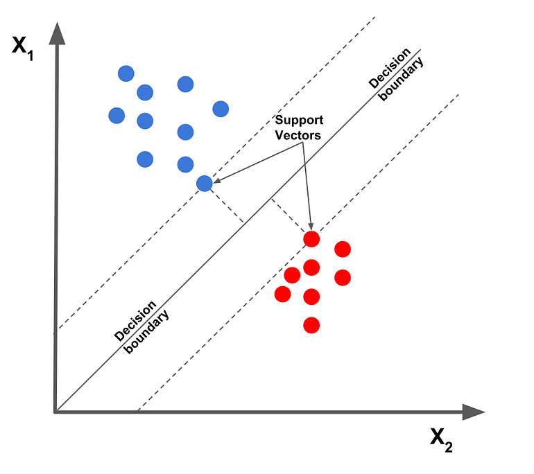
The Hyperplane: In geometry, it is an n-dimensional generalization of a plane, a subspace with one less dimension(n-1) than its origin space. In one-dimensional space, it is a point, In two-dimensional space it is a line, In three-dimensional space, it is an ordinary plane, in four or more dimensional spaces, it is then called a ‘Hyperplane’.
The Hyperplane is simply a concept that separates an n-dimensional space into two groups/halves. In machine learning terms, it is a form of a decision boundary that algorithms like the Support Vector Machine uses to classify or separate data points. There are two parts to it, the negative side hyperplane and the positive part hyperplane, where data points/instances can lie on either part, signifying the group/class they belong to.
Margin: This is the distance between the decision boundary at both sides and the nearest/closest support vectors. It can also be defined as the shortest distance between the hyperplane and the support vectors with weight w, and bias b.
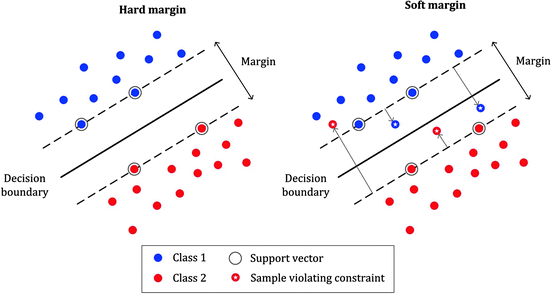
Hard Margin: This is the type of margin used for linearly separable data points in the Support vector machine. Just as the name, ‘Hard Margin’, it is very rigid in classification, hence can result in overfitting. It works best when the data is linearly separable without outliers and a lot of noise.
Soft Margin: This is the type of margin used for non-linearly separable data points. As the name literally implies, it is less rigid than the Hard-margin. It is robust to outliers and allows misclassifications. However, it can also result to underfitting in some cases.
The Kernel Trick: Kernels or Kernel Functions are methods with which linear classifiers such as SVM use to classify non-linearly separable data points. This is done by representing the data points in a higher-dimensional space than its original. For example, a 1D data can be represented as a 2D data in space, a 2D data can be represented as a 3D data et cetera. So why is it called a ‘kernel trick’? SVM cleverly re-represents non-linear data points using any of the kernel functions in a way that it seems the data have been transformed, then finds the optimal separating hyperplane. However, in reality, the data points still remain the same, they have not actually been transformed. This is why it is called a ‘kernel Trick’.
A trick indeed. Don’t you agree?
The kernel trick offers a way to calculate relationships between data points using kernel functions, and represent the data in a more efficient way with less computation. Models that use this technique are called ‘kernelized models’.
There are several functions SVM uses to perform this task. Some of the most common ones are:
Polynomial Kernel Function: This transforms data points by using the dot product and transforming data to an ‘n-dimension’, n could be any value from 2, 3 et cetera, i.e the transformation will be either a squared product or higher. Therefore representing data in higher-dimensional space using the new transformed points.
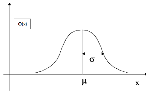
The Radial Basis Function(RBF): This function behaves like a ‘weighted nearest neighbor model’. It transforms data by representing in infinite dimensions, then using the weighted nearest neighbor (observation with the most influence on the new data point) for classification. The Radial function can be either Gaussian or Laplace. This is dependent on a hyperparameter known as gamma. This is the most commonly used kernel.
The Sigmoid Function: also known as the hyperbolic tangent function(Tanh), finds more application in neural networks as an activation function. This function is used in image classification.
The Linear Kernel: Used for linear data. This just simply represents the data points using a linear relationship.
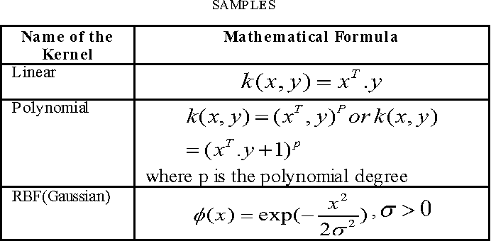
For Polynomial kernel, x and y represent the classes of observations, K represents the polynomial coefficient and p represents the degree of the polynomial. Both k and p are calculated using the cross-validation.
For Radial Basis kernel, the formula represented above is the Gaussian RBF, the representation is as follows:
The C-parameter: This is a regularization parameter used to prevent overfitting. It is inversely related to the Margin, such that if a larger C value is chosen, the margin is smaller, and if a smaller C value is chosen the margin is larger. It aids with the trade-off between bias and variance. SVM just like most machine learning algorithms has to deal with this as well.
After knowing all the terms of support vector machine, it is easy to understand support vector machine (SVM).
Support Vector Machine (SVM)
Support Vector Machine algorithm focuses on finding a hyperplane in an N-dimensional space (N-the number of features) that distinctly classifies the data points.
To classify the data points, there are many possible hyperplanes that could be chosen. Our objective is to find a plane that has the maximum margin, i.e the maximum distance between data points of classes. Maximizing the margin distance provides some reinforcement so that future data points can be classified with more confidence.
Support vectors are data points that are closer to the hyperplane and influence the position and orientation of the hyperplane. Using these support vectors, we maximize the margin of the classifier. Deleting the support vectors will change the position of the hyperplane. These are the points that help us build our SVM.
Advantages of Support Vector Machine:
- The SVM algorithm has a feature to ignore outliers and find the hyper-plane that has the maximum margin. Hence, we can say, SVM classification is robust to outliers.
- SVM works relatively well when there is a clear margin of separation between classes.
- SVM is more effective in high dimensional spaces.
- SVM is relatively memory efficient.
Disadvantages of Support Vector Machine:
- SVM algorithm is not suitable for large data sets.
- SVM does not perform very well when the data set has more noise i.e. target classes are overlapping.
- As the support vector classifier works by putting data points, above and below the classifying hyperplane there is no probabilistic explanation for the classification.
Kernel SVM
When classifying the data points using SVM is not possible since the data points are not linearly separable in 2D or there exist no hyperplane to separate them in 3D, then we use Kernel SVM.
Working of Kernel SVM:
- Map a lower dimension set of data points using a mapping function to one higher dimension where they are separated.
- Fit a line or hyperplane as per requirement to separate those points.
- Again project the same data points to lower dimensions.
Advantages of Kernel Support Vector Machine:
- The kernel trick is real strength of SVM. With an appropriate kernel function, we can solve any complex problem.
- It scales relatively well to high dimensional data.
- Risk of overfitting is less.
Disadvantages of Kernel Support Vector Machine:
- Choosing a good kernel function is not easy.
- Longer training time for large datasets.
- Difficult to understand and interpret the final model.
- Highly compute intensive.
0 Response to "Support Vector Machine"
Post a Comment