Recurrent Neural Networks (RNN)

What Is a Recurrent Neural Network (RNN)?

RNN works on the principle of saving the output of a particular layer and feeding this back to the input in order to predict the output of the layer.

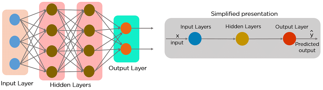
Below is how you can convert a Feed-Forward Neural Network into a Recurrent Neural Network:

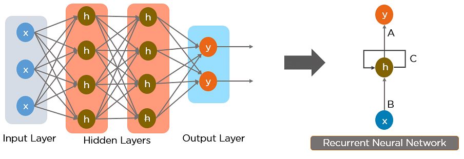
The nodes in different layers of the neural network are compressed to form a single layer of recurrent neural networks. A, B, and C are the parameters of the network.

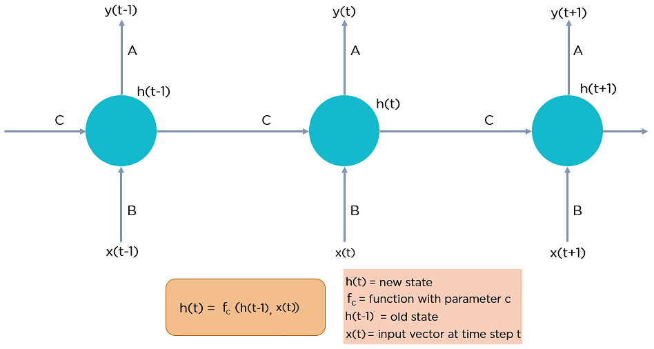
Here, “x” is the input layer, “h” is the hidden layer, and “y” is the output layer. A, B, and C are the network parameters used to improve the output of the model. At any given time t, the current input is a combination of input at x(t) and x(t-1). The output at any given time is fetched back to the network to improve on the output.

Now that you understand what a recurrent neural network is let’s look at the different types of recurrent neural networks.

Why Recurrent Neural Networks?

RNN were created because there were a few issues in the feed-forward neural network:

• Cannot handle sequential data
• Considers only the current input
• Cannot memorize previous inputs

The solution to these issues is the RNN. An RNN can handle sequential data, accepting the current input data, and previously received inputs. RNNs can memorize previous inputs due to their internal memory.

How Does Recurrent Neural Networks Work?

In Recurrent Neural networks, the information cycles through a loop to the middle hidden layer.

The input layer ‘x’ takes in the input to the neural network and processes it and passes it onto the middle layer. 

The middle layer ‘h’ can consist of multiple hidden layers, each with its own activation functions and weights and biases. If you have a neural network where the various parameters of different hidden layers are not affected by the previous layer, ie: the neural network does not have memory, then you can use a recurrent neural network.

The Recurrent Neural Network will standardize the different activation functions and weights and biases so that each hidden layer has the same parameters. Then, instead of creating multiple hidden layers, it will create one and loop over it as many times as required. 

Feed-Forward Neural Networks vs Recurrent Neural Networks

A feed-forward neural network allows information to flow only in the forward direction, from the input nodes, through the hidden layers, and to the output nodes. There are no cycles or loops in the network. 

Below is how a simplified presentation of a feed-forward neural network looks like:

In a feed-forward neural network, the decisions are based on the current input. It doesn’t memorize the past data, and there’s no future scope. Feed-forward neural networks are used in general regression and classification problems.

Applications of Recurrent Neural Networks:

Image Captioning

RNNs are used to caption an image by analyzing the activities present.

Time Series Prediction

Any time series problem, like predicting the prices of stocks in a particular month, can be solved using an RNN.

Natural Language Processing

Text mining and Sentiment analysis can be carried out using an RNN for Natural Language Processing (NLP).

Machine Translation

Given an input in one language, RNNs can be used to translate the input into different languages as output.

Types of Recurrent Neural Networks

There are four types of Recurrent Neural Networks:

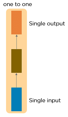
1. One to One
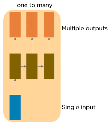
2. One to Many
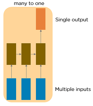
3. Many to One
4. Many to Many

One to One RNN

This type of neural network is known as the Vanilla Neural Network. It's used for general machine learning problems, which has a single input and a single output.

One to Many RNN

This type of neural network has a single input and multiple outputs. An example of this is the image caption.

Many to One RNN

This RNN takes a sequence of inputs and generates a single output. Sentiment analysis is a good example of this kind of network where a given sentence can be classified as expressing positive or negative sentiments.

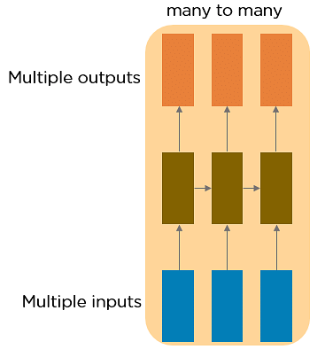
Many to Many RNN

This RNN takes a sequence of inputs and generates a sequence of outputs. Machine translation is one of the examples.

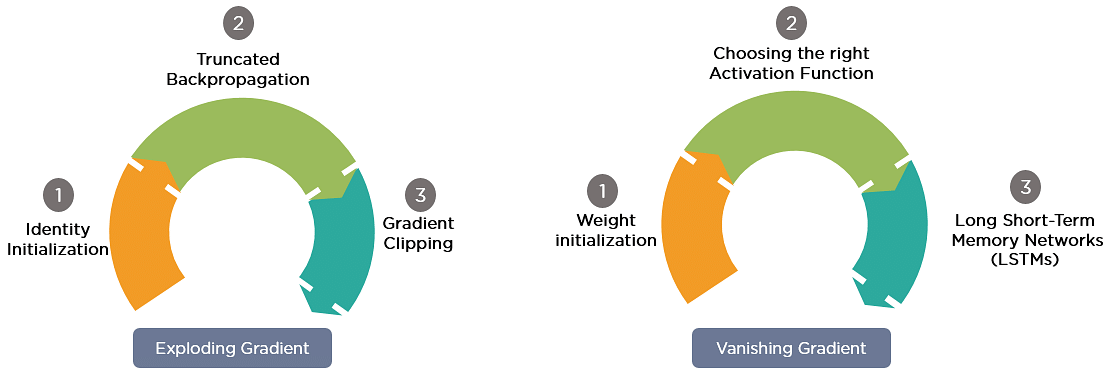
Two Issues of Standard RNNs

1. Vanishing Gradient Problem

Recurrent Neural Networks enable you to model time-dependent and sequential data problems, such as stock market prediction, machine translation, and text generation. You will find, however, RNN is hard to train because of the gradient problem.

RNNs suffer from the problem of vanishing gradients. The gradients carry information used in the RNN, and when the gradient becomes too small, the parameter updates become insignificant. This makes the learning of long data sequences difficult.

2. Exploding Gradient Problem

While training a neural network, if the slope tends to grow exponentially instead of decaying, this is called an Exploding Gradient. This problem arises when large error gradients accumulate, resulting in very large updates to the neural network model weights during the training process.

Long training time, poor performance, and bad accuracy are the major issues in gradient problems.

Gradient Problem Solutions

Now, let’s discuss the most popular and efficient way to deal with gradient problems, i.e., Long Short-Term Memory Network (LSTMs).

First, let’s understand Long-Term Dependencies.

Suppose you want to predict the last word in the text: “The clouds are in the ______.”

The most obvious answer to this is the “sky.” We do not need any further context to predict the last word in the above sentence.

Consider this sentence: “I have been staying in Spain for the last 10 years…I can speak fluent ______.”

The word you predict will depend on the previous few words in context. Here, you need the context of Spain to predict the last word in the text, and the most suitable answer to this sentence is “Spanish.” The gap between the relevant information and the point where it's needed may have become very large. LSTMs help you solve this problem.

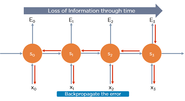
Backpropagation Through Time

Backpropagation through time is when we apply a Backpropagation algorithm to a Recurrent Neural network that has time series data as its input.

In a typical RNN, one input is fed into the network at a time, and a single output is obtained. But in backpropagation, you use the current as well as the previous inputs as input. This is called a timestep and one timestep will consist of many time series data points entering the RNN simultaneously. 

Once the neural network has trained on a timeset and given you an output, that output is used to calculate and accumulate the errors. After this, the network is rolled back up and weights are recalculated and updated keeping the errors in mind.

Long Short-Term Memory Networks (LSTM Networks)

Long Short Term Memory networks – usually just called “LSTMs” – are a special kind of RNN, capable of learning long-term dependencies. They were introduced by Hochreiter & Schmidhuber (1997), and were refined and popularized by many people in following work.1 They work tremendously well on a large variety of problems, and are now widely used.

LSTMs are explicitly designed to avoid the long-term dependency problem. Remembering information for long periods of time is practically their default behavior, not something they struggle to learn!

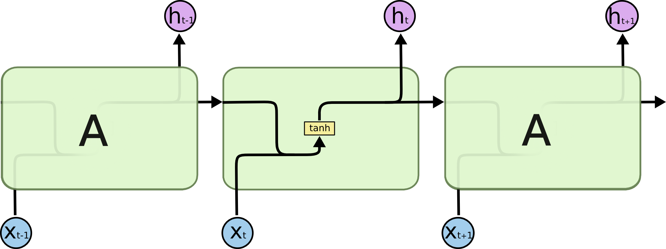
All recurrent neural networks have the form of a chain of repeating modules of neural network. In standard RNNs, this repeating module will have a very simple structure, such as a single tanh layer.

LSTMs also have this chain like structure, but the repeating module has a different structure. Instead of having a single neural network layer, there are four, interacting in a very special way.

Don’t worry about the details of what’s going on. We’ll walk through the LSTM diagram step by step later. For now, let’s just try to get comfortable with the notation we’ll be using.

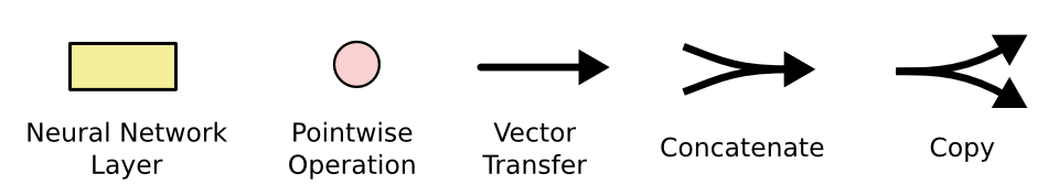
In the above diagram, each line carries an entire vector, from the output of one node to the inputs of others. The pink circles represent pointwise operations, like vector addition, while the yellow boxes are learned neural network layers. Lines merging denote concatenation, while a line forking denote its content being copied and the copies going to different locations.

The Core Idea Behind LSTMs

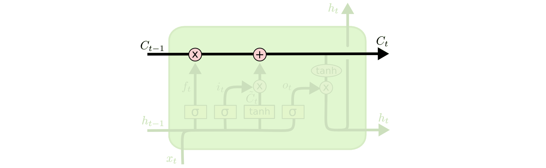
The key to LSTMs is the cell state, the horizontal line running through the top of the diagram.

The cell state is kind of like a conveyor belt. It runs straight down the entire chain, with only some minor linear interactions. It’s very easy for information to just flow along it unchanged.

The LSTM does have the ability to remove or add information to the cell state, carefully regulated by structures called gates.

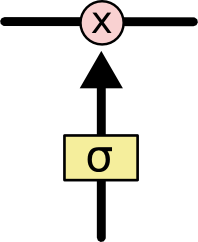
Gates are a way to optionally let information through. They are composed out of a sigmoid neural net layer and a pointwise multiplication operation.

The sigmoid layer outputs numbers between zero and one, describing how much of each component should be let through. A value of zero means “let nothing through,” while a value of one means “let everything through!”

An LSTM has three of these gates, to protect and control the cell state.

Step-by-Step LSTM Walk Through

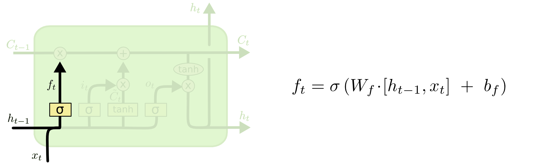
The first step in our LSTM is to decide what information we’re going to throw away from the cell state. This decision is made by a sigmoid layer called the “forget gate layer.” It looks at ht−1$h_{t-1}$ and xt$x_t$, and outputs a number between 0$0$ and 1$1$ for each number in the cell state Ct−1$C_{t-1}$. A 1$1$ represents “completely keep this” while a 0$0$ represents “completely get rid of this.”

Let’s go back to our example of a language model trying to predict the next word based on all the previous ones. In such a problem, the cell state might include the gender of the present subject, so that the correct pronouns can be used. When we see a new subject, we want to forget the gender of the old subject.

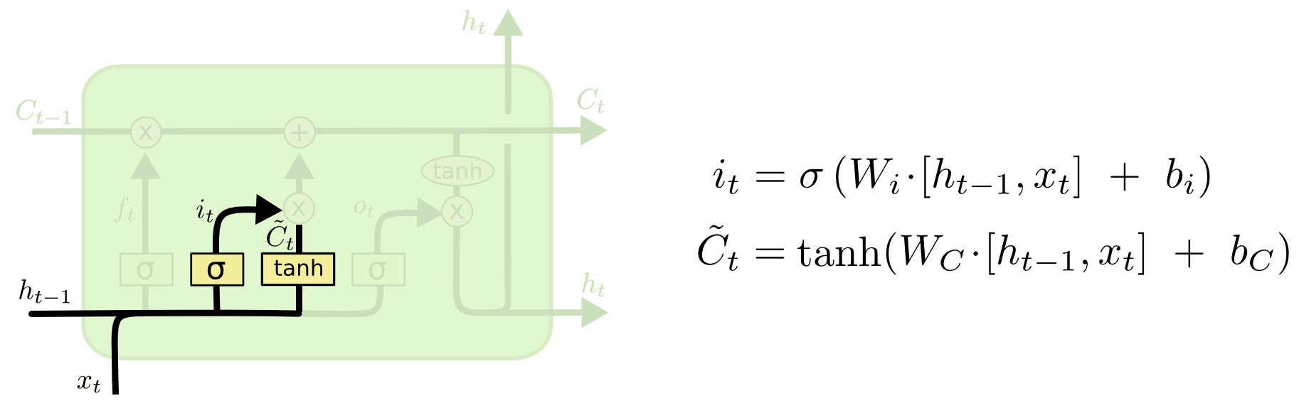
The next step is to decide what new information we’re going to store in the cell state. This has two parts. First, a sigmoid layer called the “input gate layer” decides which values we’ll update. Next, a tanh layer creates a vector of new candidate values, C~t${\tilde{C}}_t$, that could be added to the state. In the next step, we’ll combine these two to create an update to the state.

In the example of our language model, we’d want to add the gender of the new subject to the cell state, to replace the old one we’re forgetting.

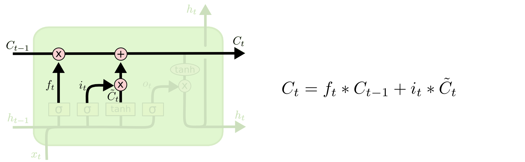
It’s now time to update the old cell state, Ct−1$C_{t-1}$, into the new cell state Ct$C_t$. The previous steps already decided what to do, we just need to actually do it.

We multiply the old state by ft$f_t$, forgetting the things we decided to forget earlier. Then we add it∗C~t$i_t\ast {\tilde{C}}_t$. This is the new candidate values, scaled by how much we decided to update each state value.

In the case of the language model, this is where we’d actually drop the information about the old subject’s gender and add the new information, as we decided in the previous steps.

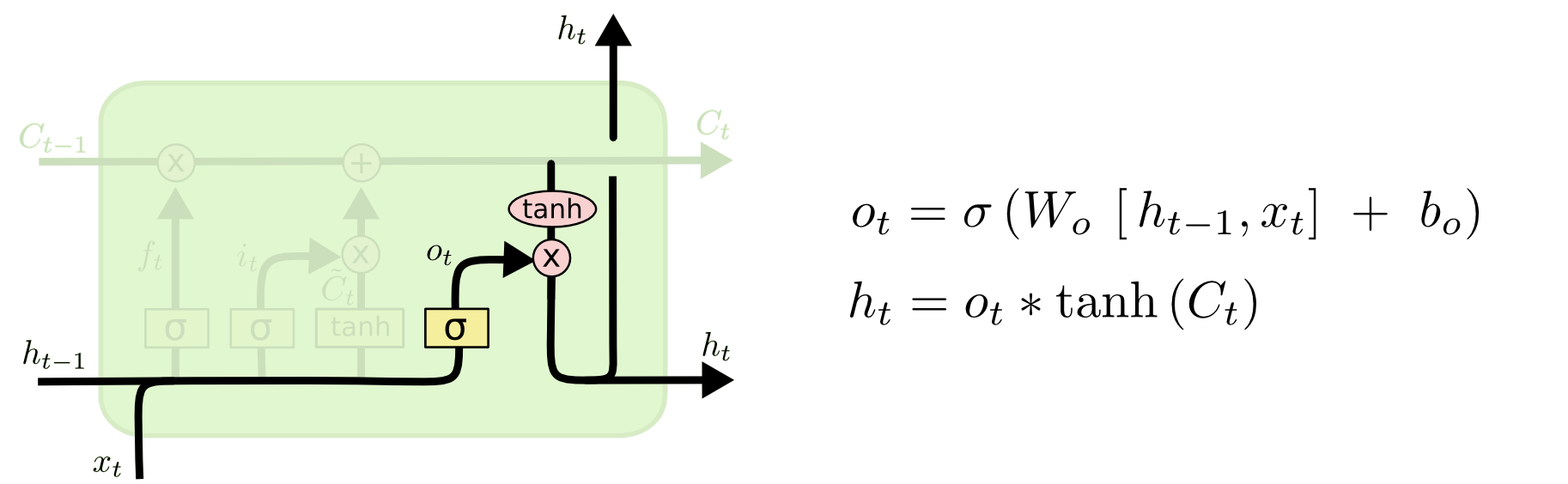
Finally, we need to decide what we’re going to output. This output will be based on our cell state, but will be a filtered version. First, we run a sigmoid layer which decides what parts of the cell state we’re going to output. Then, we put the cell state through tanh$\tanh$ (to push the values to be between −1$-1$ and 1$1$) and multiply it by the output of the sigmoid gate, so that we only output the parts we decided to.

For the language model example, since it just saw a subject, it might want to output information relevant to a verb, in case that’s what is coming next. For example, it might output whether the subject is singular or plural, so that we know what form a verb should be conjugated into if that’s what follows next.

Variants on Long Short Term Memory

What I’ve described so far is a pretty normal LSTM. But not all LSTMs are the same as the above. In fact, it seems like almost every paper involving LSTMs uses a slightly different version. The differences are minor, but it’s worth mentioning some of them.

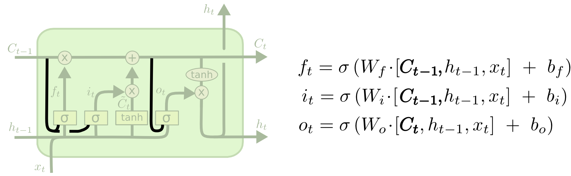
One popular LSTM variant, introduced by Gers & Schmidhuber (2000), is adding “peephole connections.” This means that we let the gate layers look at the cell state.

The above diagram adds peepholes to all the gates, but many papers will give some peepholes and not others.

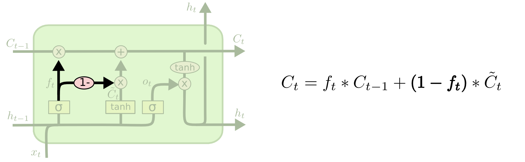
Another variation is to use coupled forget and input gates. Instead of separately deciding what to forget and what we should add new information to, we make those decisions together. We only forget when we’re going to input something in its place. We only input new values to the state when we forget something older.

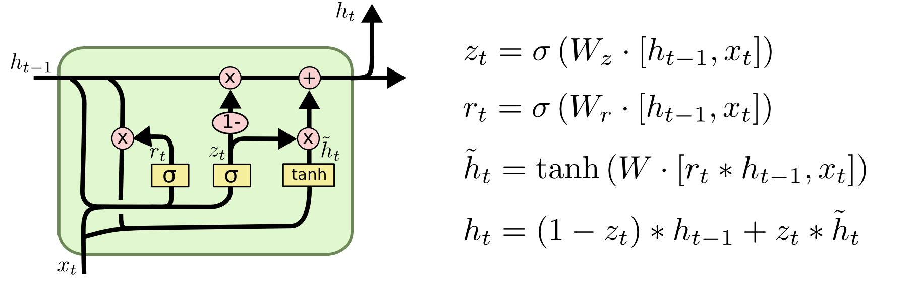
A slightly more dramatic variation on the LSTM is the Gated Recurrent Unit, or GRU, introduced by Cho, et al. (2014). It combines the forget and input gates into a single “update gate.” It also merges the cell state and hidden state, and makes some other changes. The resulting model is simpler than standard LSTM models, and has been growing increasingly popular.

These are only a few of the most notable LSTM variants. There are lots of others, like Depth Gated RNNs by Yao, et al. (2015). There’s also some completely different approach to tackling long-term dependencies, like Clockwork RNNs by Koutnik, et al. (2014).

Which of these variants is best? Do the differences matter? Greff, et al. (2015) do a nice comparison of popular variants, finding that they’re all about the same. Jozefowicz, et al. (2015) tested more than ten thousand RNN architectures, finding some that worked better than LSTMs on certain tasks.

Conclusion:

Written down as a set of equations, LSTMs look pretty intimidating. Hopefully, walking through them step by step in this essay has made them a bit more approachable.

LSTMs were a big step in what we can accomplish with RNNs. It’s natural to wonder: is there another big step? A common opinion among researchers is: “Yes! There is a next step and it’s attention!” The idea is to let every step of an RNN pick information to look at from some larger collection of information. For example, if you are using an RNN to create a caption describing an image, it might pick a part of the image to look at for every word it outputs. In fact, Xu, et al. (2015) do exactly this – it might be a fun starting point if you want to explore attention! There’s been a number of really exciting results using attention, and it seems like a lot more are around the corner.

Source:

simplilearn

colah.github.io

***Thank You***

Share this post